Answer

Generic Enquiry unable to get YTD values for invoices when pivot table created

  • August 21, 2025
  • 2 replies
  • 58 views

Forum|alt.badge.img

Hi folks,

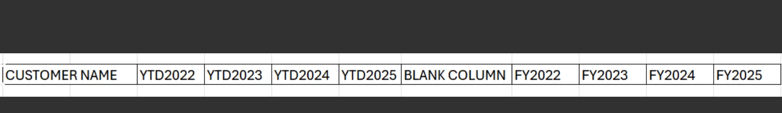
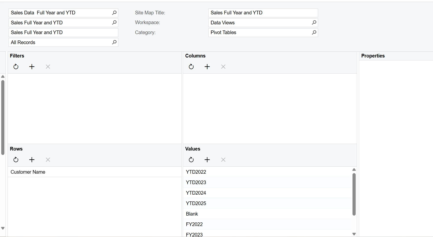
I want to create a pivot from Generic enquiry where I want to do the below image have FY and YTD values. I have already created the GI but the YTD values and sometimes even the FY values are not correct. I am not sure what my formula can improve the result intended on the Pivot table is as follows:

My formula for FY2022 is as below (Using AU financial year July to June):

=Round(IIF(( [ARTran.TranDate] > Cdate('2021-06-30')) and ([ARTran.TranDate] < Cdate('2022-07-01')),[ARTran.CuryExtPrice],0),2)

Formula for YTD is as below:

=Round(IIF(( [ARTran.TranDate] > Cdate('2021-06-30')) and ([ARTran.TranDate] < Dateadd(Today(),'y',-4)),[ARTran.CuryExtPrice],0),2)

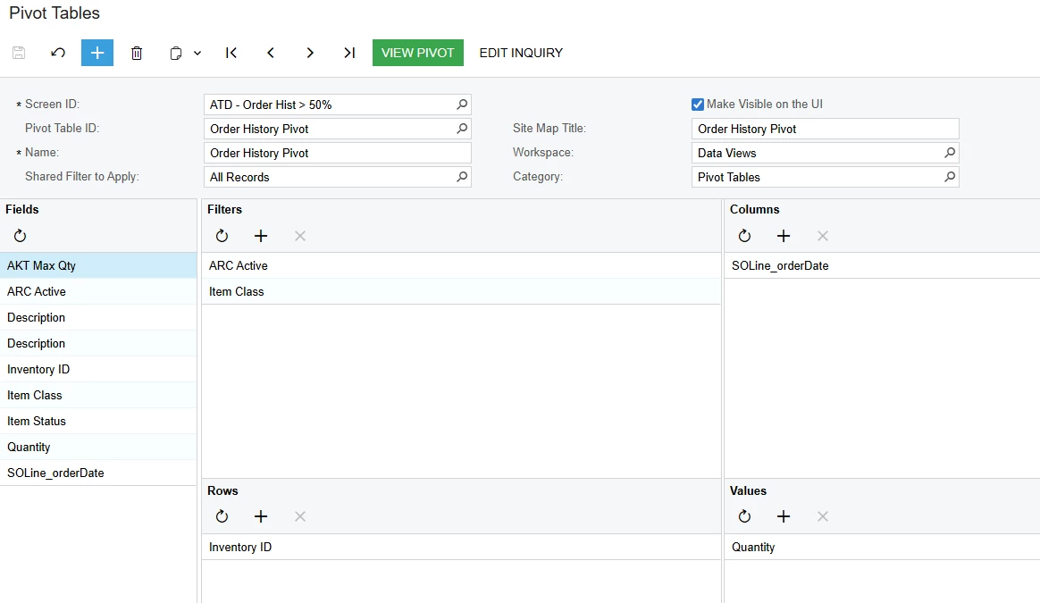
I have attached my GI as well:

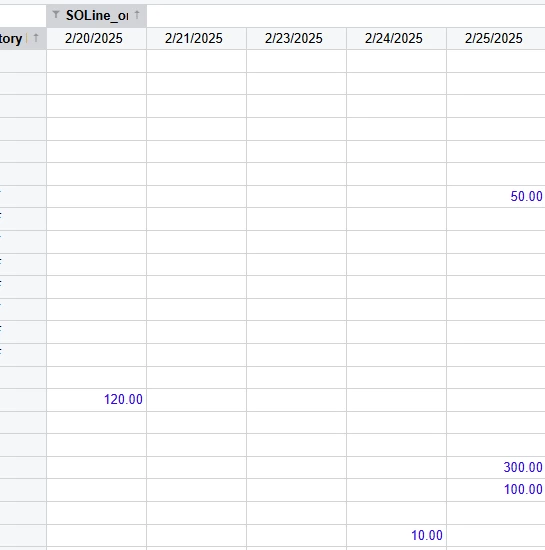
Pivot table is as below:


Any help or tips would be appreciated.

Best answer by amitkaryekar

I worked it out the main issue was only with the Formula the pivoting of the information worked well.

For YTD 2022 the formula used was as below:

=Round(IIF(( [ARTran.TranDate] > Cdate('2021-06-30')) and ([ARTran.TranDate] < Dateadd(Today(),'y',-4)),[ARTran.CuryExtPrice],0),2)


For full FY 2022 it was: 

=Round(IIF(( [ARTran.TranDate] > Cdate('2021-06-30')) and ([ARTran.TranDate] < Cdate('2022-07-01')),[ARTran.CuryExtPrice],0),2)


The pivoting of data is giving what I wanted. The only downside of it every financial year this will be required to be manually changed increasing the number by 1 for the negative figures aka YTD formula.


2 replies

Forum|alt.badge.img

You have no columns in that pivot so it isn’t going to work very well.

Usually, I would have the Customer down the side and Year across the top with the values (count or sum) (ex: Count # of orders, Sum order total). 

Example (filters are optional):
 

Result:


Looking at the GI, I don’t see how we can get the value into the column with the way you broke it out into different data points.

Usually we would do a YTD column, and a FY column, then the YTD and FY value.

So your table would look like:

         | YTD | YTDval | FY | FYval
ABC | 2022 | $100  |
QRS | 2022 | $250  |
XYZ | 2023 | $999 |
...

Then you put YTD and FY in the columns
YTDval and FYval in the Values and you get your results.

Try the attached.  I would validate the iif statements, but they appeared to work for me.


Forum|alt.badge.img
  • Author
  • Varsity I
  • Answer
  • August 21, 2025

I worked it out the main issue was only with the Formula the pivoting of the information worked well.

For YTD 2022 the formula used was as below:

=Round(IIF(( [ARTran.TranDate] > Cdate('2021-06-30')) and ([ARTran.TranDate] < Dateadd(Today(),'y',-4)),[ARTran.CuryExtPrice],0),2)


For full FY 2022 it was: 

=Round(IIF(( [ARTran.TranDate] > Cdate('2021-06-30')) and ([ARTran.TranDate] < Cdate('2022-07-01')),[ARTran.CuryExtPrice],0),2)


The pivoting of data is giving what I wanted. The only downside of it every financial year this will be required to be manually changed increasing the number by 1 for the negative figures aka YTD formula.